Demonstration of extended time-delayed feedback control on Hopf normal form
Author: Jan Sieber
Consider the Hopf normal form with single control input


(thus, ![$\partial_2f(x,0)=b=[1,1]^T$](HopfExample_eq14010628513759378264.png) .) We construct time-delayed feedback control of the form
.) We construct time-delayed feedback control of the form
![$$ u(t)=K(x(t))[\tilde x(t)-x(t)] $$](HopfExample_eq14060456685127297670.png)
where (both,  and
and  have two components)

The bifurcation diagram and the stability of the system with delay are computed using DDE-Biftool version 3.1, available from
https://sourceforge.net/projects/ddebiftool/files/dde_biftool_v3.1.zip/download
This demo is used as an illustrative example in
Sieber: Generic stabilisability for time-delayed feedback control, Preprint download at http://arxiv.org/abs/1508.05671
Contents
- Code
- Preparation: add path and define right-hand side
- Contruct bifurcation diagram
- Plot bifurcation diagram
- Construct gains for control and compute stability for controlled periodic orbit
- Plot of gains K as constructed
- Illustration of spectrum for controlled system
- Zoom in
- How does the true x-dependent gain look like?
Code
Preparation: add path and define right-hand side
Modify the path below to lead to the local ddebiftool folders.
clear
close all
addpath('../dde_biftool/ddebiftool');
addpath('../dde_biftool/ddebiftool_utilities');
hopf=@(x,p,u)[...
    p*x(1,:)-x(2,:)+x(1,:).*(x(1,:).^2+x(2,:).^2)+u;...
    p*x(2,:)+x(1,:)+x(2,:).*(x(1,:).^2+x(2,:).^2)+u];
funcs=set_funcs(...
    'sys_rhs',@(xx,p)etdf_controlled_rhs(xx,p,hopf),...
    'sys_tau',@()[],...
    'x_vectorized',true);
Contruct bifurcation diagram
Continue equilibria  initially in
  and branch off at Hopf bifurcation at
  . Then continue family of periodic orbits, and check its stability (it is unstable).
[stbr,suc]=SetupStst(funcs,'x',[0;0],'parameter',-0.2,'contpar',1,'dir',1,'step',1e-1);
display(suc)
stbr.method.continuation.plot=0;
stbr=br_contn(funcs,stbr,4);
[nunst_stst,~,~,stbr.point]=GetStability(stbr,'funcs',funcs);
suc =
     1
[pbr,suc]=SetupPsol(funcs,stbr,find(nunst_stst==2,1,'first'),'radius',0.05,'min_bound',[1,-0.5]);
pbr.method.continuation.plot=0;
pbr=br_contn(funcs,pbr,20);
[nunst_per,~,~,pbr.point]=GetStability(pbr,'funcs',funcs,'exclude_trivial',true);
BR_CONTN warning: boundary hit.
Plot bifurcation diagram
x_eq=arrayfun(@(p)p.x(1),stbr.point);
p_eq=[stbr.point.parameter];
x_per=arrayfun(@(p)max(p.profile(1,:)),pbr.point);
p_per=[pbr.point.parameter];
floq_per=arrayfun(@(p)max(abs(p.stability.mu)),pbr.point);
T_per=[pbr.point.period];
figure(1);clf
subplot(1,2,1);
plot(p_eq,x_eq,'.-',p_per,x_per,'o-');
xlabel('p');ylabel('amplitude x_1');
legend('eqilibrium','periodic orbits');
title('Bifurcation diagram')
subplot(1,2,2);
plot(p_per,log(floq_per)./T_per,'.-');
xlabel('p');ylabel('Floquet exponent (log(Multiplier)/period');
title('Stability')

Construct gains for control and compute stability for controlled periodic orbit
The function etdf_control remeshes the time point mesh along the orbit (to discretize the short large near-impulse of feedback control Then it recomputes the orbit using the new mesh (with p_correc), computes the gains using the asymptotic formula by Brunovsky'69. The gains  are chosen such that the eigenvalues of
  are placed on a circle of radious
  .
.
Time of control input is interval ![$[0,\delta]$](HopfExample_eq16457202413066742610.png) (controlled by optional parameter 't').
(controlled by optional parameter 't').
clear pcorrected spec gain
epsilon=0.005;
for i=length(pbr.point)-1:-1:1
    [pcorrected(i),spec(:,i),gain(:,i)]=etdf_control(hopf,pbr,'point',i+1,...
    't',0,'delta',1e-4,'epsilon',epsilon,'rho',0.1);
end
display(spec(1:3,:),'dominant eigenvalues of controlled system')
dominant eigenvalues of controlled system =
  Columns 1 through 2
       1.0001 +          0i            1 +          0i
      0.99526 +  0.0011534i      0.99531 +  0.0012293i
      0.99526 -  0.0011534i      0.99531 -  0.0012293i
  Columns 3 through 4
            1 +          0i            1 +          0i
      0.99536 +  0.0013055i      0.99547 +  0.0014587i
      0.99536 -  0.0013055i      0.99547 -  0.0014587i
  Columns 5 through 6
            1 +          0i            1 +          0i
      0.99565 +  0.0016865i      0.99596 +  0.0019707i
      0.99565 -  0.0016865i      0.99596 -  0.0019707i
  Columns 7 through 8
            1 +          0i            1 +          0i
      0.99643 +  0.0022525i      0.99702 +  0.0024355i
      0.99643 -  0.0022525i      0.99702 -  0.0024355i
  Columns 9 through 10
            1 +          0i            1 +          0i
       0.9976 +  0.0024396i      0.99778 +          0i
       0.9976 -  0.0024396i      0.99767 +   0.002641i
Plot of gains K as constructed
figure(3);clf
plot(p_per(2:end),gain,'.-');
set(gca,'ylim',max(abs(gain(:,end)))*[-1,1],'xlim',[min(p_per),0]);
legend('gain K_1','gain K_2');
xlabel('p');
grid on
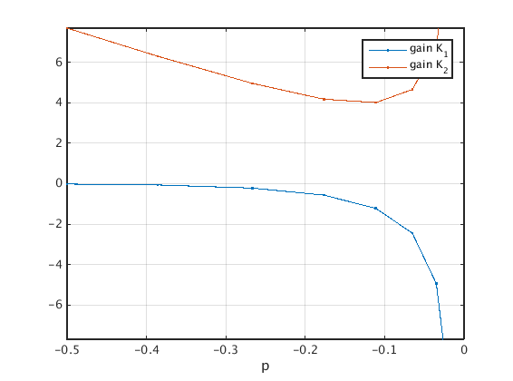
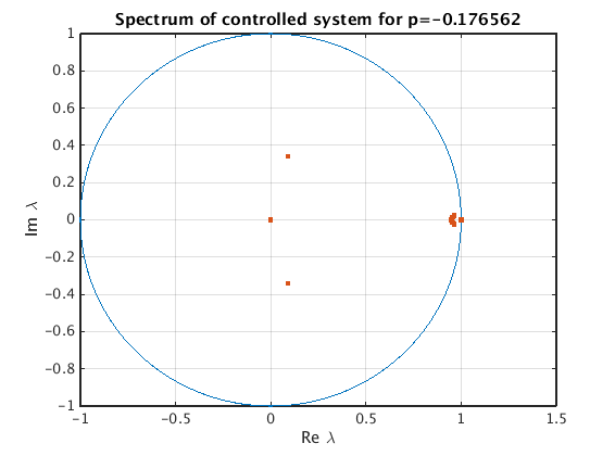
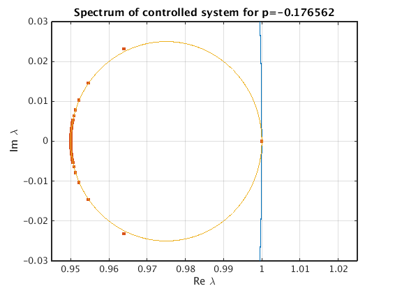
Illustration of spectrum for controlled system
for periodic orbit near p=-0.2
[~,ind]=min(abs(p_per+0.2));
epsilon=0.05;
[pt0,spec0,gain0,Ksmooth]=etdf_control(hopf,pbr,'point',ind,...
    't',0,'delta',5e-3,'epsilon',epsilon,'rho',0.1);
figure(4);clf
deco={'markersize',10};
plot(cosd(0:360),sind(0:360),real(spec0),imag(spec0),'.',deco{:});
grid on
xlabel('Re \lambda');
ylabel('Im \lambda');
title(sprintf('Spectrum of controlled system for p=%g',pt0.parameter));
drawnow
Zoom in
hold on
plot(1-epsilon/2+epsilon/2*cosd(0:360),epsilon/2*sind(0:360));
set(gca,'xlim',[1-epsilon*1.1,1+epsilon/2],'ylim',epsilon*0.6*[-1,1]);
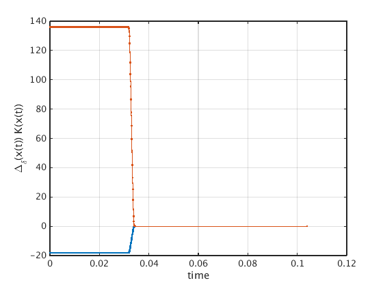
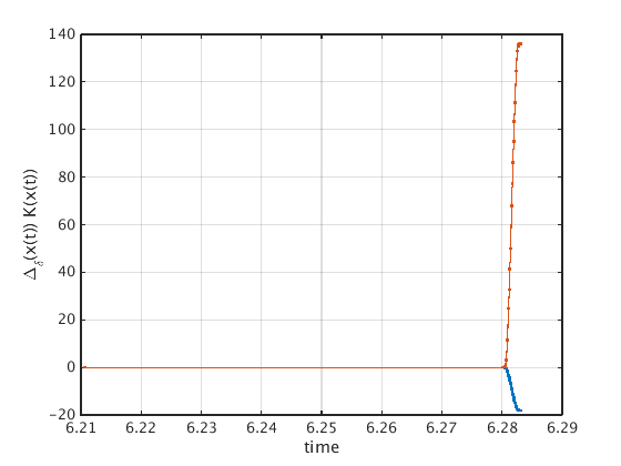
How does the true x-dependent gain look like?
The control is only applied in a small area of size delta and scaled by 1/delta.
figure(5);clf
K=Ksmooth(pt0.profile);
ind=find(all(abs(K)<1e-4),1,'first')+2;
plot(pt0.mesh(1:ind)*pt0.period,K(:,1:ind),'.-');
grid on;
xlabel('time');
ylabel('\Delta_\delta(x(t)) K(x(t))');
figure(6);clf
ind=find(all(abs(K)<1e-4),1,'last')-2;
plot(pt0.mesh(ind:end)*pt0.period,K(:,ind:end),'.-');
grid on;
xlabel('time');
ylabel('\Delta_\delta(x(t)) K(x(t))');