Demonstration of extended time-delayed feedback control on excited pendulum

Author: Jan Sieber

We consider a parametrically excited pendulum. The pendulum is driven at a frequency $\omega$ close to its 1:2 resonance. At some forcing amplitude the trivial (hanging-down) solution becomes unstable and a period-two oscillation around the hanging-down state branches off in a period doubling. For $\omega<2$ this period-doubled branch is unstable with a single unstable Floquet multiplier larger than unity.

Periodic orbits with an odd number of Floquet multipliers larger than one in periodically forced systems can usually not be stabilised with (extended) time-delayed feedback. The approach below circumvents this restriction by formulating the forcing as an autonomous Hopf normal form (Stuart-Landau) oscillator coupling into the pendulum equation (this is usually also done in an experimental implementation):

$\ddot \theta=-\gamma \dot \theta-(1+p_1 y) \sin \theta +2 u$

$y'= c p_2 y-\omega z - c y (y^2+z^2) +u$

$z'= \omega y + c p_2 z - c z (y^2+z^2) +u$

where $\gamma=0.1$ (damping), $c=0.1$ (attraction rate of periodic orbit in auxilliary oscillator $(y,z)$ ) and $\omega=1.8$ . The control input is linear through $\partial_2f(x,0)=b=(0,2,1,1)^T$ . The extended time-delayed feedback control is of the form

$u(t)=K(x(t))[\tilde x(t)-x(t)]$

$\tilde x(t)=(1-\varepsilon) \tilde x(t-T) + \varepsilon x(t-T)$

where both, $x(t)$ and $\tilde x(t)$ have four components: $\theta$ , $\dot\theta$ , $y$ and $z$ . In a practical experiment the above control would likely require two inputs: real-time torque control at the pivot of the pendulum and a a real-time modification of the (eg) actuator creating the periodic forcing.

The bifurcation diagram and the stability of the system with delay are computed using DDE-Biftool version 3.1, available from

https://sourceforge.net/projects/ddebiftool/files/dde_biftool_v3.1.zip/download

Code
Preparation: add path and define right-hand side
Contruct bifurcation diagram
Increase forcing oscillator amplitude to 1
Increase forcing of pendulum
Branch off at period doubling
Plot bifurcation diagram
Construct gains for control and compute stability for controlled periodic orbit
Plot of gains K as constructed
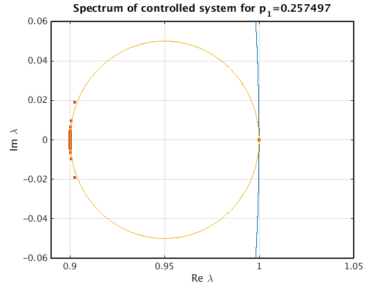
Illustration of spectrum for controlled system
Zoom in
How does the true x-dependent gain look like?

Code

Preparation: add path and define right-hand side

x is $(\theta,\dot\theta,y,z)$ and the parameter set p is $(p-1,p_2)$ . Modify the path below to lead to the local ddebiftool folders.

clear
close all
addpath('../dde_biftool/ddebiftool');
addpath('../dde_biftool/ddebiftool_utilities');
damping=0.1;
omega=1.8;
c=0.1;
pendulum=@(x,p,u)[...
    x(2,:);...
    -damping*x(2,:)-(1+p(1)*x(3,:)).*sin(x(1,:))+2*u;...
    c*p(2)*x(3,:)-omega*x(4,:)-c*x(3,:).*(x(3,:).^2+x(4,:).^2)+u;...
    omega*x(3,:)+c*p(2)*x(4,:)-c*x(4,:).*(x(3,:).^2+x(4,:).^2)+u];
funcs=set_funcs(...
    'sys_rhs',@(xx,p)etdf_controlled_rhs(xx,p,pendulum),...
    'sys_tau',@()[],...
    'x_vectorized',true);

Contruct bifurcation diagram

Continue equilibria $x=(0,0,0,0)^T$ initially in $p_2$ and branch off at Hopf bifurcation at $p_2=0$ ( $p_1$ , the forcing amplitue is 0 initially). Then continue the family of stable periodic orbits (which are trivial in|theta|: x(1)=x(2)=0) until $p_2=1$ .

[stbr,suc]=SetupStst(funcs,'x',[0;0;0;0],'parameter',[0,-0.2],...
    'contpar',2,'dir',2,'step',1e-1);
display(suc)
stbr.method.continuation.plot=0;
stbr=br_contn(funcs,stbr,5);
[nunst_stst,~,~,stbr.point]=GetStability(stbr,'funcs',funcs);

suc =

     1

Increase forcing oscillator amplitude to 1

note that forcing enters the pendulum with prefactor p(1)

[oscillator_up,suc]=SetupPsol(funcs,stbr,find(nunst_stst==2,1,'first'),...
    'radius',0.05,'max_bound',[2,1]);
display(suc)
oscillator_up.method.continuation.plot=0;
oscillator_up=br_contn(funcs,oscillator_up,20);

suc =

     1

BR_CONTN warning: boundary hit.

Increase forcing of pendulum

Now we vary $p_1$ , the forcing amplitude of the pendulum, increasing it from $0$ until we obseve a period doubling bifurcation (which occurs below $p_1=1$ ). The solution is still trivial in $\theta$ .

[trivial,suc]=ChangeBranchParameters(funcs,oscillator_up,...
    length(oscillator_up.point),'contpar',1,'dir',1,'step',0.1,'max_bound',[1,1]);
display(suc)
trivial=br_contn(funcs,trivial,100);
[nunst_triv,~,~,trivial.point]=GetStability(trivial,'funcs',funcs,...
    'exclude_trivial',true);

suc =

     1

BR_CONTN warning: boundary hit.

Branch off at period doubling

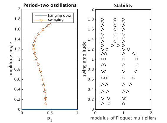
The period doubling is subcritical such that the emerging period-two oscillation (corresponding to a swinging around the hanging-down position) is unstable. The swinging solution folds in a saddle-node bifurcation, becoming stable at some $p_{1,\mathrm{fold}}$ .

ind_branch=find(nunst_triv==1,1,'first');
[swing,suc]=DoublePsol(funcs,trivial,ind_branch,'max_step',[0,0.1],...
    'max_bound',[1,trivial.point(ind_branch).parameter(1)+0.1],'radius',0.1);
display(suc)
swing=br_contn(funcs,swing,100);
[nunst_swing,dom,~,swing.point]=GetStability(swing,'funcs',funcs,'exclude_trivial',true);

suc =

     1

BR_CONTN warning: boundary hit.

Plot bifurcation diagram

x_triv=arrayfun(@(p)max(abs(p.profile(1,:))),trivial.point);
p_triv=arrayfun(@(p)p.parameter(1),trivial.point);
x_swing=arrayfun(@(p)max(p.profile(1,:)),swing.point);
p_swing=arrayfun(@(p)p.parameter(1),swing.point);
floq_swing=cell2mat(arrayfun(@(p)p.stability.mu,swing.point,'uniformoutput',false));
T_swing=[swing.point.period];
figure(1);clf;
subplot(1,2,1);
plot(p_triv,x_triv,'.-',p_swing,x_swing,'o-');
xlabel('p_1');ylabel('amplitude angle');
legend('hanging down','swinging');
title('Period-two oscillations')
subplot(1,2,2);
plot(abs(floq_swing),x_swing,'ko');
ylabel('swing amplitude');xlabel('modulus of Floquet multipliers');
title('Stability')

Construct gains for control and compute stability for controlled periodic orbit

The function etdf_control remeshes the time point mesh along the orbit (to discretize the short large near-impulse of feedback control with a finer mesh). Then it recomputes the orbit using the new mesh (with p_correc), and computes the gains using the asymptotic formula by Brunovsky'69. The gains $K_0$ are chosen such that the eigenvalues of $P_0\exp(b(0)K_0^T)$ are placed on a circle of radious $(1-\varepsilon)/2$ .

The time of control input is the interval $[0,\delta]$ (controlled by optional parameter 't').

orbits=find(nunst_swing==1); % find unstable periodic orbits
clear pcorrected spec gain
epsilon=0.1;
for i=length(orbits):-1:1
    [pcorrected(i),spec(:,i),gain(:,i)]=etdf_control(pendulum,swing,...
        'point',orbits(i),...
    't',0,'delta',1e-4,'epsilon',epsilon,'rho',0.1,'n1',5,'n_change',5,'n0',10);
end
display(spec(1:3,:),'dominant eigenvalues of controlled system')

dominant eigenvalues of controlled system =

  Columns 1 through 4

   1.0000 + 0.0000i   1.0000 + 0.0000i   1.0000 + 0.0000i   1.0000 + 0.0000i
   0.8999 + 0.0197i   0.9027 + 0.0189i   0.9032 + 0.0187i   0.9033 + 0.0187i
   0.8999 - 0.0197i   0.9027 - 0.0189i   0.9032 - 0.0187i   0.9033 - 0.0187i

  Columns 5 through 8

   1.0000 + 0.0000i   1.0000 + 0.0000i   1.0000 + 0.0000i   1.0000 + 0.0000i
   0.9034 + 0.0186i   0.9034 + 0.0186i   0.9034 + 0.0186i   0.9034 + 0.0186i
   0.9034 - 0.0186i   0.9034 - 0.0186i   0.9034 - 0.0186i   0.9034 - 0.0186i

  Columns 9 through 10

   1.0000 + 0.0000i   1.0000 + 0.0000i
   0.9032 + 0.0187i   0.9026 + 0.0189i
   0.9032 - 0.0187i   0.9026 - 0.0189i

Plot of gains K as constructed

figure(2);clf
plot(x_swing(orbits),gain,'.-');
set(gca,'ylim',max(abs(gain(:)))*[-1,1],'xlim',[0,max(x_swing(orbits))]);
legend('gain K_1','gain K_2','gain K_3','gain K_4');
xlabel('swing amplitude');
grid on

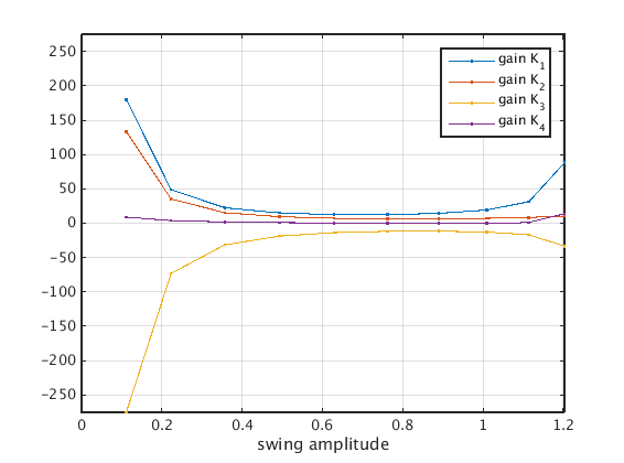
Illustration of spectrum for controlled system

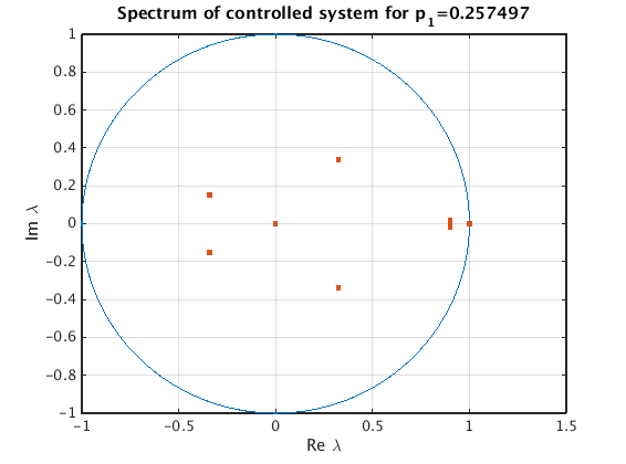
for periodic orbit with amplitude near xmax=1

[~,ind]=min(abs(x_swing-1));
epsilon=0.1;
[pt0,spec0,gain0,Ksmooth]=etdf_control(pendulum,swing,'point',ind,...
    't',0,'delta',5e-4,'epsilon',epsilon,'rho',0.1);

figure(2);clf
deco={'markersize',10};
plot(cosd(0:360),sind(0:360),real(spec0),imag(spec0),'.',deco{:});
grid on
xlabel('Re \lambda');
ylabel('Im \lambda');
title(sprintf('Spectrum of controlled system for p_1=%g',pt0.parameter(1)));
drawnow

Zoom in

hold on
plot(1-epsilon/2+epsilon/2*cosd(0:360),epsilon/2*sind(0:360));
set(gca,'xlim',[1-epsilon*1.1,1+epsilon/2],'ylim',epsilon*0.6*[-1,1]);

How does the true x-dependent gain look like?

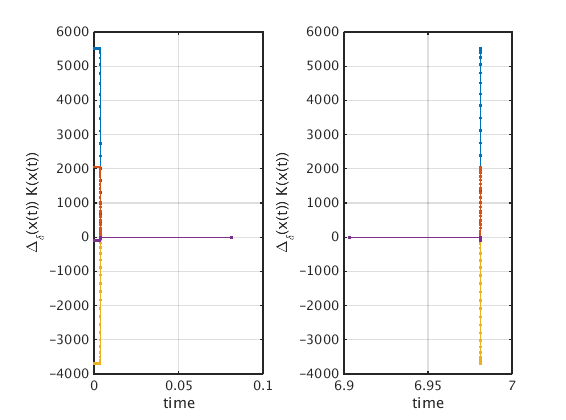
The control is only applied in a small area of size delta and scaled by 1/delta.

figure(3);clf
subplot(1,2,1);
K=Ksmooth(pt0.profile);
ind=find(all(abs(K)<1e-4),1,'first')+2;
plot(pt0.mesh(1:ind)*pt0.period,K(:,1:ind),'.-');
grid on;
xlabel('time');
ylabel('\Delta_\delta(x(t)) K(x(t))');
subplot(1,2,2);
ind=find(all(abs(K)<1e-4),1,'last')-2;
plot(pt0.mesh(ind:end)*pt0.period,K(:,ind:end),'.-');
grid on;
xlabel('time');
ylabel('\Delta_\delta(x(t)) K(x(t))');